Methanol gas synthetic images

In general endmembres extracted from a cube give usefull information but only some endmembers can be used at the classification step. In fact, many things can influence a HSI cube analysis. For this example we take a cube that is very unmixing friendly.

Figure 1 show the object, a small methanol burner. Methanol gas exit the burner. The cube is acquired in the VLW range of infrared, between 867 to 1288 wavenumber (cm-1) (7.76 to 11.54 micrometer) and it have 165 bands. The instrument used to acquire the data come from the Telops compagny. IR spectra are characteristic for chemical compounds, and their intensities are proportional to the concentration. It is what we show here. Unmixing give a fine-grained overview of the concentration.

The first step consist to extract the endmembers. The algorithm used is NFINDR with the initial working set initialized with ATGP. One of the good thing with using ATGP to create the initial working set is that this made NFINDR deterministic. Running it again with the same parameters give the same endmembers set. It is helpfull when we compare different result sets obtained with different parametrization. Figure 2 present the result set obtained by running NFINDR. For this case, twelve endmembers extracted was a good compromise. They give the information needed.

Figure 1, a small methanol burner.

Figure 2, the twelve endmembers extracted.

The second step consist to generate the abundance maps from the extracted endmembers. To present the result, the twelve abundance maps are grouped by related field: the burner (figure 3), the gas escaping the burner by the side (figure 4), the gas escaping the burner by the top (figure 5) and the backgournd (figure 6). The standard interpretation for the gas leaving by the side is a reflection of the gas leaving by the top on the burner’s metallic casing. Is it a reflection or the unmixing can detect the gas leaving by the side, I don’t no. But, a combination of both is a good hypothesis.

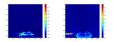
Figure 3, abundance maps related to the burner.

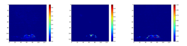
Figure 4, abundance maps related to gas leaving the burner by the side (or a reflection).

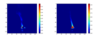
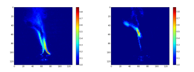
Figure 5, abundance maps related to gas leaving the burner by the top.

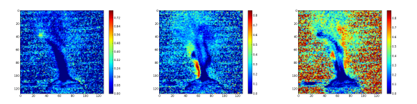
Figure 6, background abundance maps.

Finally, the synthetic images are generated by first applying a threshold and after adding the related abundance maps. The figure 7 is the burner synthetic image, the figure 8 the gas leaving by the side and figure 9 by the top.

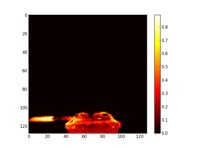
Figure 7, the burner synthetic image.

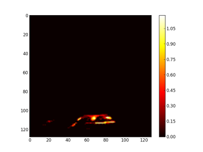
Figure 8, synthetic image of the gas leaving the burner’s side (or a reflection or both).

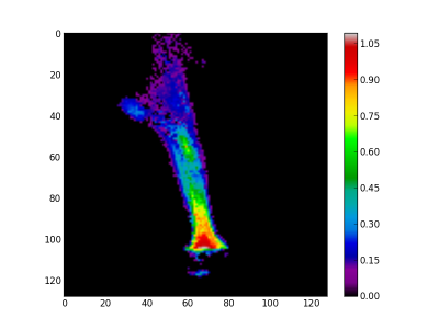
Figure 9: synthetic image of the gas leaving by the top.

The code follow:

"""
Plot abundance maps stack for the methanol gas HSI cube.
"""

from __future__ import print_function

import os
import os.path as osp
import numpy as np
import matplotlib.pyplot as plt
import pysptools.util as util
import pysptools.eea as eea
import pysptools.abundance_maps as amp


def parse_ENVI_header(head):
    ax = {}
    ax['wavelength'] = head['wavelength']
    ax['x'] = 'Wavelength - '+head['z plot titles'][0]
    ax['y'] = head['z plot titles'][1]
    return ax


def get_endmembers(data, header, result_path):
    print('Endmembers extraction with NFINDR')
    nfindr = eea.NFINDR()
    U = nfindr.extract(data, 12, maxit=5, normalize=True, ATGP_init=True)
    nfindr.plot(result_path, axes=header, suffix='gas')
    # return an array of endmembers
    return U


def gen_abundance_maps(data, U, result_path):
    print('Abundance maps generation with NNLS')
    nnls = amp.NNLS()
    amaps = nnls.map(data, U, normalize=True)
    nnls.plot(result_path, colorMap='jet', suffix='gas')
    # return an array of abundance maps
    return amaps


def plot_synthetic_gas_above(amap, colormap, result_path):
    print('Create and plot synthetic map for the gas_above')
    gas = (amap > 0.1) * amap
    stack = gas[:,:,4] + gas[:,:,5] + gas[:,:,9] + gas[:,:,10]
    plot_synthetic_image(stack, colormap, 'gas_above', result_path)


def plot_synthetic_gas_around(amap, colormap, result_path):
    print('Create and plot synthetic map for the gas_around')
    gas = (amap > 0.1) * amap
    stack = gas[:,:,6] + gas[:,:,7] + gas[:,:,8]
    plot_synthetic_image(stack, colormap, 'gas_around', result_path)


def plot_synthetic_burner(amap, colormap, result_path):
    print('Create and plot synthetic map for the burner')
    burner = (amap > 0.1) * amap
    stack = burner[:,:,2] + burner[:,:,3]
    plot_synthetic_image(stack, colormap, 'burner', result_path)


def plot_synthetic_image(image, colormap, desc, result_path):
    plt.ioff()
    img = plt.imshow(image, interpolation='none')
    img.set_cmap(colormap)
    plt.colorbar()
    fout = osp.join(result_path, 'synthetic_{0}.png'.format(desc))
    plt.savefig(fout)
    plt.clf()


if __name__ == '__main__':
    # Load the cube
    data_path = os.environ['PYSPTOOLS_DATA']
    home = os.environ['HOME']

    sample = 'burner.hdr'
    data_file = osp.join(data_path, sample)
    data, header = util.load_ENVI_file(data_file)

    result_path = osp.join(home, 'results')

    if osp.exists(result_path) == False:
        os.makedirs(result_path)

    axes = parse_ENVI_header(header)

    # Telops cubes are flipped left-right
    # Flipping them again restore the orientation
    data = np.fliplr(data)

    U = get_endmembers(data, axes, result_path)
    amaps = gen_abundance_maps(data, U, result_path)
    # best color maps: hot and spectral
    plot_synthetic_gas_above(amaps, 'spectral', result_path)
    plot_synthetic_gas_around(amaps, 'hot', result_path)
    plot_synthetic_burner(amaps, 'hot', result_path)