Smokestack
Note
Coming with the version 0.13.1, this example use NormXCorr instead of SAM. For the cube in study, NormXCorr is less sensitive to the parametrization than SAM is. The classification results are more stable.
This example follows the same pattern than the examples 2 and 3 but for one interesting add-on. As from the version 0.10, the two endmembers extraction algorithms, ATGP and FNINDR, can extract from a region of interest (ROI) and not all the cube, as it is actually the case. To control the ROI you have to define a binary mask. The binary mask is a 2D matrix, a True value at a position in the matrix means that you want to include the corresponding pixel in the endmembers search. The effluents exiting a smokestack are concentrated at the exit. We will define a small ROI just at this exit to catch the different signals that determine the gas.
Look at the Reveal Viewer screen at figure 1. The selected pixel, at the red crossbar, is located just above the smokestack where the gas emission is at the maximum. The two broad emission bands between 1075 and 1200 cm-1 correspond to the symmetric S=O stretching vibration of sulfur dioxide (SO2). The cube is acquired in the VLW range of infrared; between 867 to 1288 wavenumber (cm-1) (7.76 to 11.54 micrometer) and it have 165 bands. The instrument used to acquire the data comes from the Telops Company.

Figure 1: Reveal Viewer screen of the smokestack.
First, we extract the endmembers of the whole cube (figure 2). It will be use to compare to the ROI extracted endmembers. The spectrum tagged EM2 in green is a SO2 gas signature.
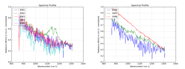
Figure 2: whole cube endmembers extracted with NFINDR, in green a SO2 signature.
Next, we make a small ROI using NormXCorr and the EM2 signature. After some tests, the threshold retained is 0.15. Figure 3 presents the binary mask.
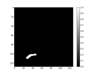
Figure 3: binary mask used to find the second endmembers set.
With the binary mask, we extract a second endmembers set. This one is composed mainly with SO2 gas signatures presents in the effluents. Look at the figure 4, the endmembers EM1 to EM7 are the SO2 the signatures.
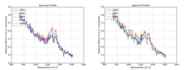
Figure 3: masked endmembers set, EM1 to EM7 are the SO2 signatures.
With this information at hand, we generate two mean images, one with NormXCorr and the other with FCLS. This is a two steps process. First, we apply a NormXCorr classification to the masked endmembers set. The upper row at figure 4 and 5 presents the results. Next, we construct the mean image by adding the EM1 to EM8 classification images and dividing the result by 8. The same process is applied using FCLS but with an important difference. To be effective, the linear unmixing model needs a good pure pixels set. A way to give it is to replace EM2 of the full cube endmembers set with each SO2 signatures given by the masked endmembers set. For each signature replacement inside the full endmembers set, we call FCLS and keep the related abundance map. In this case, this is always the second abundance map. We present these results maps in the second row of figure 4 and 5. Like with NormXCorr, we generate a mean image by adding each related abundance maps and dividing them by 8. You can see at figure 6 the two mean images.
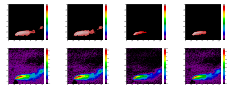
Figure 4: in red, the masked endmembers set classified with NormXCorr, in colors the same unmixed with FCLS; from left to right: spectra EM1 to EM4.

Figure 5: same as figure 4; from left to right: spectra EM5 to EM8.
Note
Transmittance is a non-linear process. The NormXCorr and FCLS mean maps are an approximation.
The mean images are an interesting achievement. The FCLS based mean image have a better resolution than the NormXCorr based image. However, the NormXCorr version takes less CPU cycle.
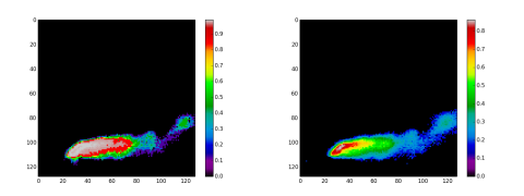
Figure 6: at left, the NormXCorr mean image, at right, the unmixed mean image.
Which one between all these SO2 signatures is a pure pixel? It is difficult to say. EM2 from the full cube endmembers set along with EM2 and EM5 from the masked endmembers set are almost identical. In addition, theirs NormXCorr classification footprints are similar to the mean NormXCorr footprint. Using the same reasoning with FCLS do not give so much evidence of which spectrum is a pure pixel.
Code follow:
"""
Plot smokestack effluents.
"""

from __future__ import print_function

import os
import os.path as osp
import pysptools.classification as cls
import matplotlib.pyplot as plt
import pysptools.util as util
import pysptools.eea as eea
import pysptools.abundance_maps as amp

import numpy as np

n_emembers = 8


def parse_ENVI_header(head):
    ax = {}
    ax['wavelength'] = head['wavelength']
    ax['x'] = 'Wavelength - '+head['z plot titles'][0]
    ax['y'] = head['z plot titles'][1]
    return ax


class Classify(object):
    """
    For this problem NormXCorr works as well as SAM
    SID was not tested.
    """

    def __init__(self, data, E, path, threshold, suffix):
        print('Classify using SAM')
        self.sam = cls.SAM()
        self.sam.classify(data, E, threshold=threshold)
        self.path = path
        self.suffix = suffix

    def get_single_map(self, idx):
        return self.sam.get_single_map(idx, constrained=False)

    def plot_single_map(self, idx):
        self.sam.plot_single_map(self.path, idx, constrained=False, suffix=self.suffix)

    def plot(self):
        self.sam.plot(self.path, suffix=self.suffix)


def get_endmembers(data, header, q, path, mask, suffix, output=False):
    print('Endmembers extraction with NFINDR')
    ee = eea.NFINDR()
    U = ee.extract(data, q, maxit=5, normalize=True, ATGP_init=True, mask=mask)
    if output == True:
        ee.plot(path, axes=header, suffix=suffix)
    return U


def get_abundance_maps(data, U, umix_source, path, output=False):
    print('Abundance maps with FCLS')
    fcls = amp.FCLS()
    amap = fcls.map(data, U, normalize=True)
    if output == True:
        fcls.plot(path, colorMap='jet', suffix=umix_source)
    return amap


def get_full_cube_em_set(data, header, path):
    """ Return a endmembers set for the full cube and a region of interest (ROI).
        The ROI is created using a small region of the
        effluents leaving near the smokestack.
    """
    # Take the endmembers set for all the cube
    U = get_endmembers(data, header, n_emembers, path, None, 'full_cube', output=True)
    # A threshold of 0.15 give a good ROI
    cls = Classify(data, U, path, 0.15, 'full_cube')
    # The endmember EM2 is use to define the region of interest
    # i.e. the effluents region of interest
    effluents = cls.get_single_map(2)
    # Create the binary mask with the effluents
    mask = (effluents > 0)
    # Plot the mask
    plot(mask, 'gray', 'binary_mask', path)
    return U, mask


def get_masked_em_set(data, header, path, mask):
    """ Return a endmembers set that belong to the ROI (mask).
    """
    # Use the mask to extract endmembers near the smokestack exit
    U = get_endmembers(data, header, n_emembers, path, mask, 'masked', output=True)
    return U


def classification_analysis(data, path, E_masked):
    # Note: the classification is done with NormXCorr instead of SAM
    # Classify with the masked endmembers set
    c = cls.NormXCorr()
    c.classify(data, E_masked, threshold=0.15)
    c.plot_single_map(path, 'all', constrained=False, suffix='masked')
    c.plot(path, suffix='masked')
    # Calculate the average image
    gas = c.get_single_map(1, constrained=False)
    for i in range(n_emembers - 1):
        gas = gas + c.get_single_map(i+2, constrained=False)
    gas = gas / n_emembers
    # and plot it
    plot(gas, 'spectral', 'mean_NormXCorr', path)


def unmixing_analysis(data, path, E_full_cube, E_masked):
    # Calculate an unmixed average image at the ROI position.
    # Each endmember belonging to E_masked takes place inside E_full_cube at
    # the ROI position. Netx, we sum the abundance maps
    # generated at this position. And finally a mean is calculated.
    for i in range(n_emembers):
        E_full_cube[1,:] = E_masked[i,:]
        amaps = get_abundance_maps(data, E_full_cube, 'masqued_{0}'.format(i+1), path, output=False)
        if i == 0:
            mask = amaps[:,:,1]
        else:
            mask = mask + amaps[:,:,1]
        plot(amaps[:,:,1], 'spectral', 'FCLS_masqued_{0}'.format(i+1), path)
    mask = mask / n_emembers
    thresholded = (mask > 0.15) * mask
    plot(thresholded, 'spectral', 'mean_FCLS', path)


def plot(image, colormap, desc, path):
    plt.ioff()
    img = plt.imshow(image, interpolation='none')
    img.set_cmap(colormap)
    plt.colorbar()
    fout = osp.join(path, '{0}.png'.format(desc))
    plt.savefig(fout)
    plt.clf()


if __name__ == '__main__':
    plt.ioff()

    # Load the cube
    data_path = os.environ['PYSPTOOLS_DATA']
    home = os.environ['HOME']

    sample = 'Smokestack1.hdr'
    data_file = osp.join(data_path, sample)
    data, header = util.load_ENVI_file(data_file)

    result_path = osp.join(home, 'results')

    if osp.exists(result_path) == False:
        os.makedirs(result_path)

    axes = parse_ENVI_header(header)

    # Telops cubes are flipped left-right
    # Flipping them again restore the orientation
    data = np.fliplr(data)

    U_full_cube, mask = get_full_cube_em_set(data, axes, result_path)
    U_masked = get_masked_em_set(data, axes, result_path, mask)
    classification_analysis(data, result_path, U_masked)
    unmixing_analysis(data, result_path, U_full_cube, U_masked)